Durbin and Koopman: Box-Jenkins Examples¶

See Durbin and Koopman (2012), Chapter 8.4

%matplotlib inline

import numpy as np
import pandas as pd
from dismalpy import ssm
import matplotlib.pyplot as plt

# Get the basic series
dinternet = np.array(pd.read_csv('data/internet.csv').diff()[1:])

# Remove datapoints
missing = np.r_[6,16,26,36,46,56,66,72,73,74,75,76,86,96]-1
dinternet[missing] = np.nan

# Statespace
mod = ssm.SARIMAX(dinternet, order=(1,0,1))
res = mod.fit()
print res.summary()

                           Statespace Model Results
==============================================================================
Dep. Variable:                      y   No. Observations:                   99
Model:               SARIMAX(1, 0, 1)   Log Likelihood                -225.770
Date:                Mon, 21 Sep 2015   AIC                            457.541
Time:                        14:49:44   BIC                            465.326
Sample:                             0   HQIC                           460.691
                                 - 99
Covariance Type:                  opg
==============================================================================
                 coef    std err          z      P>|z|      [0.025      0.975]
------------------------------------------------------------------------------
ar.L1          0.6562      0.092      7.156      0.000       0.476       0.836
ma.L1          0.4878      0.111      4.394      0.000       0.270       0.705
sigma2        10.3402      1.569      6.590      0.000       7.265      13.416
===================================================================================
Ljung-Box (Q):                         nan   Jarque-Bera (JB):                  nan
Prob(Q):                               nan   Prob(JB):                          nan
Heteroskedasticity (H):                nan   Skew:                              nan
Prob(H) (two-sided):                   nan   Kurtosis:                          nan
===================================================================================

Warnings:
[1] Covariance matrix calculated using the outer product of gradients.

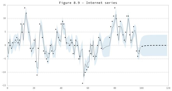
# In-sample one-step-ahead predictions, and out-of-sample forecasts
nforecast = 20
predict = res.get_prediction(end=mod.nobs + nforecast)
idx = np.arange(len(predict.predicted_mean))
predict_ci = predict.conf_int(alpha=0.5)

# Graph
fig, ax = plt.subplots(figsize=(12,6))
ax.xaxis.grid()
ax.plot(dinternet, 'k.')

# Plot
ax.plot(idx[:-nforecast], predict.predicted_mean[:-nforecast], 'gray')
ax.plot(idx[-nforecast:], predict.predicted_mean[-nforecast:], 'k--', linestyle='--', linewidth=2)
ax.fill_between(idx, predict_ci[:, 0], predict_ci[:, 1], alpha=0.15)

ax.set(title='Figure 8.9 - Internet series');