Representation in Python
The basic guiding principle for translation of state space models into Python is to allow users to focus on the specification aspect of their model rather than on the machinery of efficient and accurate filtering and smoothing computation. To do this, it applies the programmatic technique of object oriented programming (OOP). While a full description and motivation of OOP is beyond the scope of this paper, one of the primary benefits for our purposes is that it facilitates organization and prevents the writing and rewriting of the same or similar code. This feature is quite attractive in general, but as will be shown below, state space models fit particularly well into - and reap substantial benefits from - the object oriented paradigm. Once a state space model has been specified, filtering, smoothing, a large part of parameter estimation, and some postestimation results are standard; they depend only on the generic form of the model given in (?) rather than the specializations found in, for example, (?), (?), and (?)).
The Python programming language is general-purpose, interpreted, dynamically typed, and high-level. Relative to other programming languages commonly used for statistical computation, it has both strengths and weaknesses. It lacks the breadth of available statistical routines present in the R programming language, but instead features a core stack of well-developed scientific libraries. Since it began life as a general purpose programming language, it lacks the native understanding of matrix algebra which makes MATLAB so easy to begin working with (these features are available, but are provided by the the Numeric Python (NumPy) and Scientific Python (SciPy) libraries) but has more built-in features for working with text, files, web sites, and more. All of Python, R, and MATLAB feature excellent graphing and plotting features and the ability to integrate compiled code for faster performance.
Of course, anything that can be done in one language can in principle be done in many others, so familiarity, style, and tradition play a substantial role in determining which language is used in which discipline. There is much to recommend R, MATLAB, Stata, Julia, and other languages. Nonetheless, it is hoped that this paper will not only show how state space models can be specified and estimated in Python, but also introduce some of the powerful and elegent features of Python that make it a strong candidate for consideration in a wide variety of statistical computing projects.
Object oriented programming
What follows is a brief description of the concepts of object oriented programming. The content follows [31], which may be consulted for more detail. The Python Language Reference may be consulted for details on the implementation and syntax of object oriented programming specific to Python.
Objects are “collections of operations that share a state” ([31]). Another way to put it is that objects are collections of data (the state) along with functions that operate on or otherwise make use of that data (the operations). In Python, the data held by an object are called its attributes and the operations are called its methods. An example of an object is a point in the Cartesian plane, where we suppose that the “state” of the point is its coordinates in the plane and there are two methods, one to change its \(x\)-coordinate to \(x + dx\), and one to change the \(y\)-coordinate to \(y + dy\).
Classes are “templates from which objects can be created ... whereas the
[attributes of an] object represent actual variables, class
[attributes] are potential, being instantiated only when an object is
created” (Ibid.). The point object described above could be written in Python
code in the following way: first by defining a Point class:
# This is the class definition. Object oriented programming has the concept
# of inheritance, whereby classes may be "children" of other classes. The
# parent class is specified in the parentheses. When defining a class with
# no parent, the base class `object` is specified instead.
class Point(object):

    # The __init__ function is a special method that is run whenever an
    # object is created. In this case, the initial coordinates are set to
    # the origin. `self` is a variable which refers to the object instance
    # itself.
    def __init__(self):
        self.x = 0
        self.y = 0

    def change_x(self, dx):
        self.x = self.x + dx

    def change_y(self, dy):
        self.y = self.y + dy
and then by creating a point_object object by instantiating that class:
# An object of class Point is created
point_object = Point()

# The object exposes it's attributes
print(point_object.x)  # 0

# And we can call the object's methods
# Notice that although `self` is the first argument of the class method,
# it is automatically populated, and we need only specify the other
# argument, `dx`.
point_object.change_x(-2)
print(point_object.x)  # -2
Object oriented programming allows code to be organized hierarchically through the concept of class inheritance, whereby a class can be defined as an extension to an existing class. The existing class is called the parent and the new class is called the child. [31] writes “inheritance allows us to reuse the behavior of a class in the definition of new classes. Subclasses of a class inherit the operations of their parent class and may add new operations and new [attributes]”.
Through the mechanism of inheritance, a parent class can be defined with a set of generic functionality, and then many child classes can subsequently by defined with specializations. Each child thus contains both the generic functionality of the parent class as well as its own specific functionality. Of course the child classes may have children of their own, and so on.
As an example, consider creating a new class describing vectors in
\(\mathbb{R}^2\). Since a vector can be described as an ordered pair of
coordinates, the Point class defined above could also be used to describe
vectors and allow users to modify the vector using the change_x and
change_y methods. Suppose that we wanted to add a method to calculate the
length of the vector. It wouldn’t make sense to add a length method to the
Point class, since a point does not have a length, but we can create a new
Vector class extending the Point class with the new method. In the code
below, we also introduce arguments into the class constructor (the __init__
method).
# This is the new class definition. Here, the parent class, `Point`, is in
# the parentheses.
class Vector(Point):

    def __init__(self, x, y):
        # Call the `Point.__init__` method to initialize the coordinates
        # to the origin
        super(Vector, self).__init__()

        # Now change to coordinates to those provided as arguments, using
        # the methods defined in the parent class.
        self.change_x(x)
        self.change_y(y)

    def length(self):
        # Notice that in Python the exponentiation operator is a double
        # asterisk, "**"
        return (self.x**2 + self.y**2)**0.5

# An object of class Vector is created
vector_object = Vector(1, 1)
print(vector_object.length())  # 1.41421356237
Returning to state space models and Kalman filtering and smoothing, the object oriented approach allows for separation of concerns, and prevents duplication of effort. The base classes contain the functionality common to all state space models, in particular Kalman filtering and smoothing routines, and child classes fill in model-specific parameters into the state space representation matrices. In this way, users need only specify the parts that are absolutely necessary and yet the classes they define contain full state space operations. In fact, many additional features beyond filtering and smoothing are available through the base classes, including methods for estimation of unknown parameters, summary tables, prediction and forecasting, model diagnostics, simulation, and impulse response functions.
Basic representation
In this section we present the first of two classes that most applications will use.
The class dismalpy.ssm.Model (referred to as simply Model in what
follows) provides a direct interface to the state space functionality described
above. Thus it requires specification of the state space matrices (i.e. the
elements from Table 1) and in return it provides a number of
built-in functions that can be called by users. The most important of these are
loglike, filter, smooth, and simulation_smoother.
The first, loglike, performs the Kalman filter recursions and returns the
joint loglikelihood of the sample. The second, filter, performs the Kalman
filter recursions and returns an object holding the full output of the filter
(see Table 2), as well as the state space representation (see
Table 1). The third, smooth, performs Kalman filtering
and smoothing recursions and returns an object holding the full output of
the smoother (see Table 3) as well as the filtering output
and the state space representation. The last, simulation_smoother, creates
a new object that can be used to create an arbitrary number of simulated state
and disturbance series (see Table 4).
As an example of the use of this class, consider the following code, which
constructs a local level model for the Nile data with known parameter values
(the next section will consider parameter estimation), and then applies the
above methods. Recall that to fully specify a state space model, all of the
elements from Table 1 must be set, and the Kalman filter must
be initialized. In the Model class, all state space elements are created
as zero matrices of the appropriate shapes, so often only the non-zero
elements need be specified. [1]
# To instantiate the object, provide the observed data (here `nile`)
# and the dimension of the state vector
nile_model_1 = dp.ssm.Model(nile, k_states=1)
# The state space representation matrices are initialized to zeros,
# and must be set to the values prescribed by the model

# The design, transition, and selection matrices are fully fixed
# by the local level model.
nile_model_1['design', 0, 0] = 1.0
nile_model_1['transition', 0, 0] = 1.0
nile_model_1['selection', 0, 0] = 1.0

# The observation and state disturbance covariance matrices are not
# in general known; here we take values from Durbin and Koopman (2012)
nile_model_1['obs_cov', 0, 0] = 15099.0
nile_model_1['state_cov', 0, 0] = 1469.1

# Initialize as approximate diffuse, and "burn" the first
# loglikelihood value
nile_model_1.initialize_approximate_diffuse()
nile_model_1.loglikelihood_burn = 1
Notice that the approach did not create a subclass. Instead, it instantiated
the Model class directly as an object which was then manipulated. In this
case, this method was more convenient, although an equivalent approach
utilizing a subclass could have been used. For parameter estimation, below, the
approach utilizing a subclass is almost always preferrable. The following code
therefore specifies the same model as above, but utilizing a subclass approach.
# Create a new class with parent dp.ssm.Model
class BaseLocalLevel(dp.ssm.Model):

    # Recall that the constructor (the __init__ method) is
    # always evaluated at the point of object instantiation
    # Here we require a single instantiation argument, the
    # observed dataset, called `endog` here.
    def __init__(self, endog):

        # This calls the constructor of the parent class. This
        # line is analogous to the line
        # `nile_model_1 = dp.ssm.Model(nile, k_states=1)` in
        # previous example
        super(BaseLocalLevel, self).__init__(endog, k_states=1)

        # The below code mirrors the previous example, except
        # that instead of the object instance `nile_model_1`, we
        # use the self-referential object instance `self`.

        # Here we only set the generically known elements
        self['design', 0, 0] = 1.0
        self['transition', 0, 0] = 1.0
        self['selection', 0, 0] = 1.0

        self.initialize_approximate_diffuse()
        self.loglikelihood_burn = 1

# Instantiate a new object
nile_model_2 = BaseLocalLevel(nile)

# Now, set the covariance matrices to the values
# specific to the nile model
nile_model_2['obs_cov', 0, 0] = 15099.0
nile_model_2['state_cov', 0, 0] = 1469.1
Either of the above approaches fully specifies the local level state space
model. At our disposal now are the methods provided by the Model class.
They can be applied as follows.
First, the loglike method returns a single number.
# Evaluate the joint loglikelihood of the data
print(nile_model_1.loglike())  # -632.537695048
# or, we could equivalently use the second model with identical results
print(nile_model_2.loglike())  # -632.537695048
The filter method returns an object from which filter output can be
retrieved.
# Retrieve filtering output
nile_filtered_1 = nile_model_1.filter()
# print the filtered estimate of the unobserved level
print(nile_filtered_1.filtered_state[0])         # [1103.34  ... 798.37]
print(nile_filtered_1.filtered_state_cov[0, 0])  # [14874.41  ... 4032.16]
The smooth method returns an object from which smoother output can be
retrieved.
# Retrieve smoothing output
nile_smoothed_1 = nile_model_1.smooth()
# print the smoothed estimate of the unobserved level
print(nile_smoothed_1.smoothed_state[0])         # [1107.20 ... 798.37]
print(nile_smoothed_1.smoothed_state_cov[0, 0])  # [4015.96  ... 4032.16]
Finally the simulation_smoother method returns an object that can be
used to simulate state or disturbance vectors via the simulate method.
# Retrieve a simulation smoothing object
nile_simsmoother_1 = nile_model_1.simulation_smoother()
# Perform first set of simulation smoothing recursions
nile_simsmoother_1.simulate()
print(nile_simsmoother_1.simulated_state[0, :-1])  # [1000.10 ... 882.31]
# Perform second set of simulation smoothing recursions
nile_simsmoother_1.simulate()
print(nile_simsmoother_1.simulated_state[0, :-1])  # [1153.62 ... 808.44]
Fig. 4 plots the observed data, filtered series, smoothed series, and the simulated level from ten simulations, generated from the above model.
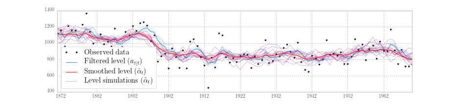
Fig. 4 Filtered and smoothed estimates and simulatations of unobserved level for Nile data.
The Model class is thus sufficient for performing filtering, smoothing,
etc. operations on a known model, but it is not convenient for the estimation
of unknown parameters. A second class with estimation in mind is described in
the following section.
| [1] | More specifically, potentially time-varying matrices are created as zero matrices of the appropriate non-time-varying shape. If a time-varying matrix is required, the whole matrix must be re-created in the appropriate time-varying shape before individual elements may be modified. |
Representation for parameter estimation
The introduction of parameter estimation into the Python representation of a
state space model will require practical implementation of the concepts that
were introduced in order to consider parameter estimation in the state space
model. These concepts are (1) the idea of a mapping from
parameter values to system matrices, and (2) the specification of initial
parameter values. Although there are many ways to implement these, what follows
is the convention used throughout; for compatibility with existing classes (for
example the maximum likelihood estimation helper class
dismalpy.ssm.MLEModel) it is recommended that users do not deviate from
them.
In the above example using the subclass approach, the fixed elements of the
state space representation were set in the class constructor (the __init__
method) and the elements corresponding to parameter values were set later. This
is the pattern that will be used; in particular we will add a new method to the
class, an update method, that will accept as its argument the full vector
of parameters \(\psi\) and will update the system matrices as appropriate.
With this we have implemented the mapping described above. Second, we will add
a new attribute to the class, called start_params, that will hold the
vector of initial parameter values. [2]
The following code re-writes the above local level implementation to use these two new features.
class LocalLevel(dp.ssm.Model):

    # Define the initial parameter vector; see update() below for a note
    # on the required order of parameter values in the vector
    start_params = [1.0, 1.0]

    # Define the fixed state space elements in the constructor
    def __init__(self, endog):
        super(LocalLevel, self).__init__(endog, k_states=1)

        self['design', 0, 0] = 1.0
        self['transition', 0, 0] = 1.0
        self['selection', 0, 0] = 1.0

        self.initialize_approximate_diffuse()
        self.loglikelihood_burn = 1

    def update(self, params):
        # Using the parameters in a specific order in the update method
        # implicitly defines the required order of parameters
        self['obs_cov', 0, 0] = params[0]
        self['state_cov', 0, 0] = params[1]
Notice that in the code above, only the fixed state space elements common to
all local level models was set in the constructor.The two variance parameters
remain to be set, using the update method, after the object is
instantiated with a specific dataset:
# Instantiate a new object
nile_model_3 = LocalLevel(nile)
# Now, update the model with the values specific to the nile model
nile_model_3.update([15099.0, 1469.1])

print(nile_model_3.loglike())  # -632.537695048

# Try updating with a different set of values, and notice that the
# evaluated likelihood changes.
nile_model_3.update([10000.0, 1.0])

print(nile_model_3.loglike())  # -687.5456216
Additional remarks
Several additional remarks are merited about the implementation that is available when using or creating subclasses of the base classes.
First, if the model is time-invariant, then a check for convergence will be
used at each step of the Kalman filter iterations. Once convergence has been
achieved, the converged state disturbance covariance matrix, Kalman gain, and
forecast error covariance matrix are used at all remaining iterations,
reducing the computational burden. The tolerance for determining convergence is
controlled by the tolerance attribute, which is initially set to
\(10^{-19}\) but can be changed by the user. For example, to disable the
use of converged values in the above Nile model one could use the code
nile_model_3.tolerance = 0.
Second, two recent innovations in Kalman filtering are available to handle
large-dimensional observations. These include the univariate filtering approach
of [18] and the collapsed approach of
[14]. The use of these approaches are
controlled by the set_filter_method method. For example, to enable
both of these approaches in the Nile model, one could use the code
nile_model_3.set_filter_method(filter_univariate=True, filter_collapsed=True)
(this is just for illustration, since of course there is only a single variable
in that model meaning that these options would have no practical effect). The
univariate filtering method is enabled by default, but the collapsed approach
is not.
Next, options to enable conservation of computer memory (RAM) are available,
and are controllable via the set_conserve_memory method. It should be noted
that the usefulness of these options depends on the analysis required by the
user, because smoothing requires all filtering values and simulation smoothing
requires all smoothing and filtering values. However, in maximum likelihood
estimation or Metropolis-Hastings posterior simulation, all that is required is
the joint likelihood value. One might enable memory conservation until
optimal parameters have been found, and then disable it so as to calculate any
filtered and smoothed values of interest. In Gibbs sampling MCMC approaches,
memory conservation is not available because the simulation smoother is
required.
Fourth, predictions and impulse response functions are immediately
available for any state space model through the filter results object (obtained
as the returned value from a filter call), through the predict and
impulse_responses methods.
Fifth, the Kalman filter (and smoothers) are fully equipped to handle missing observation data; no special code is required.
Finally, before moving on to specific parameter estimation methods, it is
important to note that the simulation smoother object created via the
simulation_smoother method generates simulations based on the state space
matrices as they are defined when the simulation is performed and not when
the simulate method is called. This will be important when considering
Gibbs sampling MCMC parameter estimation methods, below. As an illustration,
consider the following code:
# BEFORE: Perform some simulations with the original parameters
nile_model_3.update([15099.0, 1469.1])
nile_simsmoother_3.simulate()
# ...

# AFTER: Perform some new simulations with new parameters
nile_model_3.update([10000.0, 1.0])
nile_simsmoother_3.simulate()
# ...
Fig. 5 plots ten simulations generated during the BEFORE period, and ten simulations from the AFTER period. It is clear that they are simulating different series, reflecting the different parameters values in place at the time of simulation.
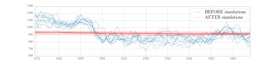
Fig. 5 Simulations of the unobserved level for Nile data under two different parameter sets.
| [2] | It may seem restrictive to require the initial parameter value to be a a class attribute, which is set to a specific value. In practice, the attribute can be replaced with a class property, allowing dynamic creation of the attribute’s value. In this way the initial parameter vector for an ARMA(p,q) model could, for example, be generated using ordinary least squares. |
Practical considerations
As described before, two practical considerations with the Kalman filter are numerical stability and performance. Briefly discussed were the availability of a square-root filter and the use of compiled computer code. In practice, the square-root filter is rarely required, and this Python implementation does not use it. One good reason for this is that “the amount of computation required is substantially larger” ([10]), and acceptable numerical stability for most models is usually achieved via forcing symmetry of the state covariance matrix (see [11], for example).
High performance is achieved primarily through the use of Cython ([3]) which allows suitably modified Python code to be compiled to C, in some cases (such as the current one) dramatically improving performance. Also, as described in the preceding section, recent advances in filtering with large-dimensional observations are available. Note that the use of compiled code for performance-critical computation is also pursued in several of the other Kalman filtering implementations mentioned in the introduction.
An additional practical consideration whenever computer code is at issue is the possibility of programming errors (“bugs”). [21] emphasize the need for tests ensuring accurate results, as well as good documentation and the availability of source code so that checking for bugs is possible. The source code for this implementation is available, with reasonably extensive inline comments describing procedures. Furthermore, even though the spectre of bugs cannot be fully exorcised, several hundred “unit tests” have been written, and are available for users to run themselves, comparing output to known results from a variety of outside sources. These tests are run continuously with the software’s development to prevent errors from creeping in.
At this point, we once again draw attention to the separation of
concerns made possible by the implementation approach pursued here. Although
writing the code for a conventional Kalman filter is relatively trivial,
writing the code for a Kalman filter, smoother, and simulation smoother using
the univariate and collapsed approaches, properly allowing for missing data,
and in a compiled language to achieve acceptable performance is not. And yet,
for models in state space from, the solution, once created, is entirely
generic. The use of an object oriented approach here is what allows users to
have the best of both worlds: classes can be custom designed using only Python
and yet they contain methods (loglike, filter, etc.) which have been
written and compiled for high performance, and tested for accuracy.
Example models
In this section, we provide code describing the example models in the previous sections. This code is provided to illustrate the above principles in specific models, and it is not necessarily the best way to estimate these models. For example, it is more efficient to develop a class to handle all ARMA(p,q) models rather than separate classes for different orders.
ARMA(1, 1) model
The following code is a straightforward translation of (?). Notice
that here the state dimension is 2 but the dimension of the state disturbance
is only 1; this is represented in the code by setting k_states=2 but
k_posdef=1. [3] Also demonstrated is the possibility of specifying the
Kalman filter initialization in the class construction call
(initialization='stationary'), since the model is assumed to be
stationary. [4]
class ARMA11(dp.ssm.Model):

    start_params = [0, 0, 1]

    def __init__(self, endog):
        super(ARMA11, self).__init__(
            endog, k_states=2, k_posdef=1, initialization='stationary')

        self['design', 0, 0] = 1.
        self['transition', 1, 0] = 1.
        self['selection', 0, 0] = 1.

    def update(self, params):
        self['design', 0, 1] = params[1]
        self['transition', 0, 0] = params[0]
        self['state_cov', 0, 0] = params[2]

# Example of instantiating a new object, updating the parameters to the
# starting parameters, and evaluating the loglikelihood
inf_model = ARMA11(inf)
inf_model.update(inf_model.start_params)
inf_model.loglike()  # -1545.0987090041408
Local level model
The class for the local level model was defined in the previous section.
Real business cycle model
The real business cycle model is specified by (?). It again has a
state dimension of 2 and a state disturbance dimension of 1, and again the
process is assumed to be stationary. Unlike the previous examples, here the
parameters of the model do not map one-to-one to elements of the system
matrices. As described in the definition of the RBC model, the thirteen
reduced form parameters found in the state space matrices are non-linear
functions of combinations of the six structural parameters. We want to set up
the model in terms of the structural parameters and use the update method
to perform the appropriate transformations to retrieve the reduced form
parameters. This is important because the theory does not allow the reduced
form parameters to vary arbitrarily; in particular, only certain combinations
of the reduced form parameters are consistent with generation through the model
from the underlying structural parameters.
Give reduced form parameters, the specification of the state space model itself is trivial, but estimation of the reduced form model requires solution of the structural model for the reduced form parameters in terms of the structural parameters. This requires the solution of a linear rational expectations model, which is beyond the scope of this paper. This particular RBC model can be solved using the method of [4]; more general solution methods exist for more general models (see for example [16] and [28]).
Regardless of the method used, for many linear (or linearized) models, the solution will be in state space form and so the state space matrices can be updated with the reduced form parameters. The following code snippet is not complete, but shows the general formulation in Python.
class SimpleRBC(dp.ssm.Model):

    start_params = [...]

    def __init__(self, endog):
        super(SimpleRBC, self).__init__(
            endog, k_states=2, k_posdef=1, initialization='stationary')

        # Initialize RBC-specific variables, parameters, etc.
        # ...

        # Setup fixed elements of the statespace matrices
        self['selection', 1, 0] = 1

    def solve(self, structural_params):
        # Solve the RBC model
        # ...

    def update(self, params):
        params = super(SimpleRBC, self).update(params, transformed)

        # Reconstruct the full parameter vector from the
        # estimated and calibrated parameters
        structural_params = ...
        measurement_variances = ...

        # Solve the model
        design, transition = self.solve(structural_params)

        # Update the statespace representation
        self['design'] = design
        self['obs_cov', 0, 0] = measurement_variances[0]
        self['obs_cov', 1, 1] = measurement_variances[1]
        self['obs_cov', 2, 2] = measurement_variances[2]
        self['transition'] = transition
        self['state_cov', 0, 0] = structural_params[...]
| [3] | The dimension of the state disturbance is named k_posdef because the
selected state disturbance vector is given not by \(\eta_t\) but by
\(R_t \eta_t\). The dimension of the selected state disturbance
vector is always equal to the dimension of the state, but the selected
state disturbance covariance matrix will be have
k_states - k_posdef zero-eigenvalues. Thus the dimension of
the state disturbance gives the dimension of the subset of the selected
state disturbance for which a positive definite covariance matrix. |
| [4] | Of course the assumption of stationarity would be violated for certain parameter values, for example if \(\phi = 1\). This has important implications for parameter estimation, where we typically want to only allow parameters inducing a stationary model, and is discussed in the specific sections on parameter estimation. |